Gaussian-Process Latent Variable Model (GPLVM) with Input Optimisation#
🌟 Motivation#
Real-world data often lies on complex, curved surfaces or manifolds in a high-dimensional space. Think of images, speech signals, or biological measurements: although high-dimensional, they typically possess a much simpler underlying structure. Can we automatically discover such a simplified, low-dimensional structure from complex data?
A powerful solution to this question is the Gaussian-Process Latent Variable Model (GPLVM):
GPLVM elegantly extends Gaussian Processes to unsupervised learning, automatically discovering low-dimensional representations.
It reveals the intrinsic structure hidden in high-dimensional observations by optimising latent input positions.
It outperforms linear methods (like PCA) in capturing nonlinear relationships and structure.
In short: GPLVM helps you “unroll” complex manifolds, simplifying data representation and interpretation.
Show code cell source
import numpy as np
import matplotlib.pyplot as plt
from sklearn.datasets import make_swiss_roll
from sklearn.decomposition import PCA
from sklearn.manifold import TSNE

# Generate smaller Swiss roll dataset for fast visualization
n_samples = 500
X, color = make_swiss_roll(n_samples, noise=0.05)
X = X[:, [0, 2, 1]]  # reorder axes for better visualization

# Apply PCA
pca = PCA(n_components=2)
X_pca = pca.fit_transform(X)

# Faster t-SNE with fewer iterations and lower perplexity
tsne = TSNE(n_components=2, init='pca', random_state=42, perplexity=20, n_iter=500)
X_tsne = tsne.fit_transform(X)

# Plot
fig = plt.figure(figsize=(15, 4))

# 3D Swiss Roll
ax = fig.add_subplot(131, projection='3d')
ax.scatter(X[:, 0], X[:, 1], X[:, 2], c=color, cmap=plt.cm.Spectral, s=10)
ax.set_title("Original 3D Swiss Roll")
ax.view_init(10, -70)

# PCA
plt.subplot(132)
plt.scatter(X_pca[:, 0], X_pca[:, 1], c=color, cmap=plt.cm.Spectral, s=10)
plt.title("PCA Projection")
plt.xlabel("PC 1")
plt.ylabel("PC 2")

# t-SNE (motivates GPLVM)
plt.subplot(133)
plt.scatter(X_tsne[:, 0], X_tsne[:, 1], c=color, cmap=plt.cm.Spectral, s=10)
plt.title("t-SNE Embedding (Nonlinear)")
plt.xlabel("Dim 1")
plt.ylabel("Dim 2")

plt.suptitle("Motivation for GPLVM: Recovering Low-Dimensional Manifolds", fontsize=14)
plt.tight_layout()
plt.subplots_adjust(top=0.85)
plt.show()
/Users/christoph/miniconda3/lib/python3.13/site-packages/sklearn/manifold/_t_sne.py:1164: FutureWarning: 'n_iter' was renamed to 'max_iter' in version 1.5 and will be removed in 1.7.
  warnings.warn(
/Users/christoph/miniconda3/lib/python3.13/site-packages/sklearn/utils/extmath.py:335: RuntimeWarning: divide by zero encountered in matmul
  Q, _ = normalizer(A @ Q)
/Users/christoph/miniconda3/lib/python3.13/site-packages/sklearn/utils/extmath.py:335: RuntimeWarning: overflow encountered in matmul
  Q, _ = normalizer(A @ Q)
/Users/christoph/miniconda3/lib/python3.13/site-packages/sklearn/utils/extmath.py:335: RuntimeWarning: invalid value encountered in matmul
  Q, _ = normalizer(A @ Q)
/Users/christoph/miniconda3/lib/python3.13/site-packages/sklearn/utils/extmath.py:336: RuntimeWarning: divide by zero encountered in matmul
  Q, _ = normalizer(A.T @ Q)
/Users/christoph/miniconda3/lib/python3.13/site-packages/sklearn/utils/extmath.py:336: RuntimeWarning: overflow encountered in matmul
  Q, _ = normalizer(A.T @ Q)
/Users/christoph/miniconda3/lib/python3.13/site-packages/sklearn/utils/extmath.py:336: RuntimeWarning: invalid value encountered in matmul
  Q, _ = normalizer(A.T @ Q)
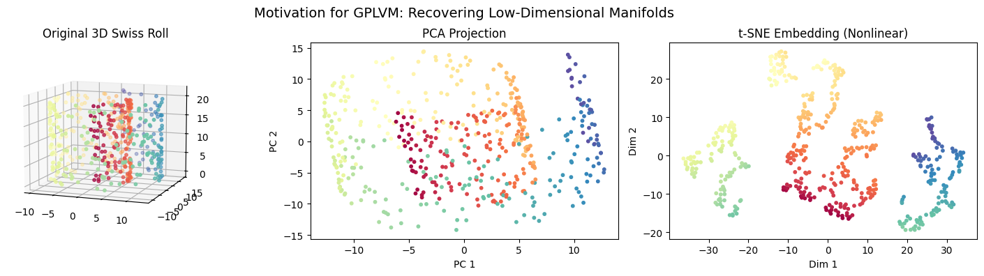
This visualization shows:
Left: the true high-dimensional manifold structure.
Middle: PCA, a linear method that fails to “unroll” the manifold.
Right: t-SNE, a nonlinear method that recovers the latent 2D structure (like GPLVM aims to do, but with a probabilistic model).
📌 What You Will Do in This Project#
Your main goal is straightforward yet powerful:
Implement a Gaussian-Process Latent Variable Model (GPLVM) to find a meaningful 2-D latent representation of the classic 3-D Swiss-roll dataset.
You will:
Implement GPLVM from scratch, using NumPy.
Optimise latent variables (input points in latent space) and kernel hyperparameters simultaneously.
Visualise your learned latent embedding clearly to show how GPLVM uncovers the underlying 2-D structure hidden in the data.
🔍 Key Concepts You’ll Master#
Through this project, you’ll build practical skills around these key ideas:
Latent Variable Modelling: Understanding how latent inputs (unobserved) can be optimised to explain complex observed data effectively.
GP Marginal Likelihood and MAP: You’ll learn how the marginal likelihood of Gaussian Processes guides simultaneous optimisation of latent variables and kernel hyperparameters.
Alternating Optimisation: Discover how to iteratively optimise latent inputs and kernel parameters to reveal meaningful low-dimensional representations.
Nonlinear Dimensionality Reduction: Compare how GPLVM performs better than linear methods (PCA), providing more interpretable embeddings.
🚧 Core Tasks (Implementation Details)#
You will practically engage with these tasks:
Latent Initialisation (PCA): Begin by initialising latent 2-D positions for your data points using PCA, providing a sensible starting point.
Alternating Optimisation: Perform iterative optimisation steps, alternating between:
Optimising latent inputs (X).
Optimising kernel hyperparameters (length-scale, signal variance, noise variance).
Visualization: Create clear visualisations of your latent embedding (2-D space) colour-coded by the height of the original Swiss-roll, showing clearly how GPLVM effectively “unrolls” the manifold.
📝 Reporting: Analysis and Insights#
Your short report (~2 pages) should focus on insightful comparisons and explanations:
Show derivation of the GPLVM.
Clearly explain why GPLVM provides a more meaningful embedding than PCA for nonlinear data like the Swiss-roll.
Visually illustrate your embedding, highlighting key structural features and smoothness of the learned representation.
Briefly discuss how optimising both inputs and kernel parameters leads to more powerful dimensionality reduction.
🚀 Stretch Goals (Optional, Advanced)#
If you’re keen to explore further, you might:
Implement back-constraints: add parametric mappings to better generalise to new data points.
Compare GPLVM embedding to other nonlinear methods such as t-SNE, highlighting differences in interpretability and manifold preservation.
📚 Resources and Support#
Starter code for data generation (Swiss-roll) and visualisation will be provided, enabling you to focus on the core GPLVM implementation.
Feel free to leverage external resources, lecture notes, and clearly documented AI-assistance.
✅ Why This Matters#
GPLVM is not just a fascinating theoretical concept; it’s highly practical and valuable in real-world contexts:
Widely used in fields such as bioinformatics, robotics, computer vision, and data visualization.
Provides deep intuition into nonlinear dimensionality reduction, latent-variable modeling, and Gaussian processes—crucial topics in modern machine learning.
Demonstrates your ability to implement complex probabilistic models, optimally position latent variables, and interpret sophisticated models visually and mathematically.
This project is an opportunity to create a standout portfolio piece and gain robust understanding and confidence in modern nonlinear probabilistic modeling.
Project Summary: Gaussian-Process Latent Variable Model (GPLVM) with Input Optimization#
(NumPy)
Item |
Details |
|---|---|
Goal |
Fit a 2-D latent representation for 3-D Swiss-roll using GPLVM MAP. |
Key ideas |
Latent \(X\) as parameters, GP marginal likelihood, alternating optimisation. |
Core tasks |
|
Report |
Show derivation of the GPLVM; explain why GPLVM can “unroll” the manifold better than PCA. |
Stretch |
Add back-constraints or compare to t-SNE. |