Bayesian Logistic Regression with Variational Inference#
🌟 Motivation#
Classification tasks are everywhere—spam filtering, image classification, medical diagnosis, and beyond. Traditional logistic regression gives us clear, interpretable classification boundaries, but there’s a critical limitation: uncertainty isn’t captured. How confident are we about predictions away from our data points? Can we quantify this uncertainty?
Bayesian logistic regression answers these questions beautifully by modeling uncertainty directly in our predictions. However, performing exact Bayesian inference is often impossible. To address this, we turn to Variational Inference (VI)—a powerful, scalable approach for approximate Bayesian inference:
VI enables practical Bayesian modeling, even in cases when exact methods (like Markov Chain Monte Carlo) become computationally prohibitive.
It provides principled uncertainty estimates alongside predictive means.
It uses optimization techniques you’re familiar with (gradient ascent) to approximate complex posterior distributions.
Show code cell source
import numpy as np
import matplotlib.pyplot as plt
from sklearn.datasets import make_moons
from sklearn.linear_model import LogisticRegression
from scipy.special import expit, entr

# Generate two-moons dataset
X, y = make_moons(n_samples=300, noise=0.2, random_state=0)

# Fit standard logistic regression for comparison
clf = LogisticRegression()
clf.fit(X, y)

# Generate grid for predictions
xx, yy = np.meshgrid(np.linspace(-2, 3, 300), np.linspace(-1.5, 2, 300))
grid = np.c_[xx.ravel(), yy.ravel()]

# Predict probabilities using logistic regression
probs = clf.predict_proba(grid)[:, 1].reshape(xx.shape)
entropy = entr(probs) + entr(1 - probs)  # predictive entropy

# Plotting
fig, ax = plt.subplots(1, 2, figsize=(12, 5))

# Decision boundary and data
ax[0].contourf(xx, yy, probs, levels=25, cmap='RdBu', alpha=0.7)
ax[0].contour(xx, yy, probs, levels=[0.5], colors='black', linewidths=1.5)
ax[0].scatter(X[:, 0], X[:, 1], c=y, cmap='bwr', edgecolor='k', s=30)
ax[0].set_title("Logistic Regression Decision Boundary")
ax[0].set_xlabel("$x_1$")
ax[0].set_ylabel("$x_2$")
ax[0].set_xlim(-2, 3)
ax[0].set_ylim(-1.5, 2)

# Entropy plot
cs = ax[1].contourf(xx, yy, entropy, levels=25, cmap='viridis')
ax[1].scatter(X[:, 0], X[:, 1], c=y, cmap='bwr', edgecolor='k', s=30, alpha=0.4)
ax[1].set_title("Predictive Entropy (Uncertainty)")
ax[1].set_xlabel("$x_1$")
ax[1].set_ylabel("$x_2$")
ax[1].set_xlim(-2, 3)
ax[1].set_ylim(-1.5, 2)
fig.colorbar(cs, ax=ax[1], label='Entropy')

plt.tight_layout()
plt.show()
/Users/christoph/miniconda3/lib/python3.13/site-packages/sklearn/utils/extmath.py:203: RuntimeWarning: divide by zero encountered in matmul
  ret = a @ b
/Users/christoph/miniconda3/lib/python3.13/site-packages/sklearn/utils/extmath.py:203: RuntimeWarning: overflow encountered in matmul
  ret = a @ b
/Users/christoph/miniconda3/lib/python3.13/site-packages/sklearn/utils/extmath.py:203: RuntimeWarning: invalid value encountered in matmul
  ret = a @ b
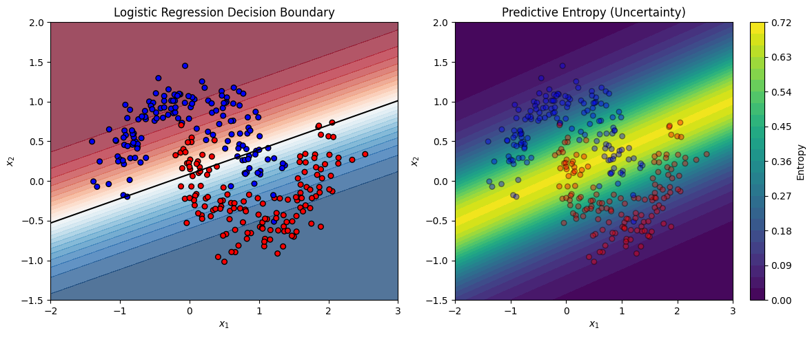
Left plot: The decision boundary learned by standard logistic regression (MLE).
Right plot: The predictive uncertainty visualized as entropy — highest far from the data, as a Bayesian model would estimate.
This illustration can serve as a baseline. You can later compare it to your Bayesian VI implementation, which should:
produce similar decision boundaries,
but show more calibrated uncertainty, especially in regions lacking data.
📌 What You Will Do in This Project#
Your clear goal is:
Implement Bayesian Logistic Regression using Variational Inference (VI) and apply it to the classic nonlinear “two moons” classification dataset.
Specifically, you’ll:
Implement a diagonal-Gaussian variational approximation \(q(\mathbf{w})\) for logistic regression.
Derive and maximize the Evidence Lower Bound (ELBO) using stochastic gradient ascent.
Visualize clearly the Bayesian decision boundary and predictive uncertainty across the data space.
🔍 Key Concepts You’ll Master#
Throughout this project, you’ll gain hands-on experience and deep understanding of:
Bayesian Classification: Moving beyond deterministic decision boundaries toward probability distributions over parameters and predictions.
Variational Inference (VI): Learning how to approximate difficult posterior distributions with simpler families (diagonal Gaussians) by maximizing the ELBO.
Evidence Lower Bound (ELBO): Understanding ELBO as a powerful and intuitive objective balancing data likelihood and model complexity.
Re-parameterization trick: Using this key computational trick to efficiently compute gradients for your stochastic gradient ascent.
🚧 Core Tasks (Implementation Details)#
You will concretely engage with these tasks:
ELBO Derivation: Derive clearly (with your own steps) the ELBO objective for Bayesian logistic regression with a Gaussian variational posterior.
Stochastic Gradient Ascent Implementation: Implement gradient-based optimization (e.g., using minibatches) to efficiently maximize your ELBO and approximate the true posterior distribution.
Visualization: Plot clearly the learned Bayesian decision boundary, and also visualize predictive uncertainty (entropy) across your feature space.
📝 Reporting: Analysis and Insights#
Your brief (~2 pages) report should include clear comparisons and intuitive insights:
Derivation of the ELBO: Derive the ELBO from first principles.
Derivation of the Gradient: Derive the gradient of the ELBO from first principles.
Deterministic vs. Bayesian Boundaries: Clearly compare standard logistic regression to Bayesian logistic regression decision boundaries, highlighting key differences.
Uncertainty Visualization: Discuss explicitly how predictive uncertainty (entropy) varies away from training data, emphasizing why this matters practically.
Insights into ELBO optimization: Briefly discuss how the ELBO changes during optimization and how the posterior uncertainty evolves.
🚀 Stretch Goals (Optional, Advanced)#
If you’re eager for additional depth, you might:
Move beyond diagonal covariance, implementing a low-rank plus diagonal full covariance variational posterior.
Compare your VI-based Bayesian logistic regression against a Laplace approximation, discussing practical trade-offs in computational complexity and quality of uncertainty estimates.
📚 Resources and Support#
Starter notebooks will be provided, including synthetic “two moons” data and basic visualization tools to help you focus on core VI implementation.
You may use external resources, lecture notes, and clearly documented AI-assisted tools in your implementation.
✅ Why This Matters#
This project positions you at the forefront of practical Bayesian machine learning and probabilistic modeling techniques:
VI is widely used for scalable Bayesian modeling in industry and academia—across fields such as NLP, computer vision, healthcare, and finance.
Understanding and implementing Bayesian logistic regression with VI equips you with practical experience, highly valued by industry and research groups.
You’ll create a visually intuitive and analytically insightful piece, perfect for your portfolio.
Project Summary: Bayesian Logistic Regression with Variational Inference#
(NumPy)
Item |
Details |
|---|---|
Goal |
Classify 2-D moons with Bayesian logistic regression using a diagonal-Gaussian variational posterior. |
Key ideas |
Laplace vs. VI, ELBO, re-parameterisation trick. |
Core tasks |
|
Report |
Show derivation of the ELBO; compare deterministic vs. Bayesian boundary; discuss uncertainty away from data. |
Stretch |
Use full-covariance q via low-rank + diag. |